Variance GWA Summary

The function summarized the variance GWA result for the given scan object.

Usage

# S3 method for class 'vGWAS'
summary(object, nrMarkers = 10, ...)

Arguments

object: a result object from vGWAS scan. It can be any list or data.frame that contains chromosome, marker.map, and p.value, with class = 'vGWAS'. See vGWAS.
nrMarkers: a numeric value giving the number of top markers to be summarized.
...: not in use

Value

a summary for viewing vGWAS result.

References

Shen, X., Pettersson, M., Ronnegard, L. and Carlborg, O. (2011): Inheritance beyond plain heritability: variance-controlling genes in Arabidopsis thaliana. PLoS Genetics, 8, e1002839.

Ronnegard, L., Shen, X. and Alam, M. (2010): hglm: A Package for Fitting Hierarchical Generalized Linear Models. The R Journal, 2(2), 20-28.

Author

Xia Shen

Examples

# \donttest{
# ----- load data ----- #
data(pheno)
data(geno)
data(chr)
data(map)
# ----- variance GWA scan ----- #
vgwa <- vGWAS(phenotype = pheno, geno.matrix = geno,
marker.map = map, chr.index = chr, pB = FALSE)
#> 
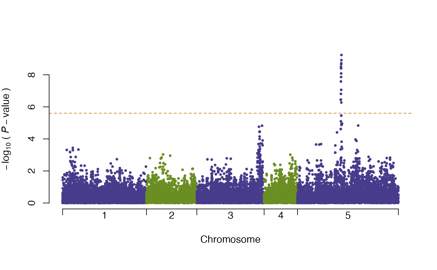
# ----- visualize the scan ----- #
plot(vgwa)
#> nominal significance threshold with Bonferroni correction for 20000 tests are calculated.

summary(vgwa)
#> [1] Top 10 markers, sorted by p-value:
#>    marker chr    map               Pval
#> 1  V16630   5 393135 0.0000000005831907
#> 2  V16627   5 392704 0.0000000012144397
#> 3  V16621   5 391781 0.0000000018983749
#> 4  V16614   5 390839 0.0000000021781079
#> 5  V16601   5 388736 0.0000000031525392
#> 6  V16609   5 390084 0.0000000039528039
#> 7  V16612   5 390492 0.0000000039528039
#> 8  V16613   5 390663 0.0000000082466233
#> 9  V16608   5 389975 0.0000000137787674
#> 10 V16598   5 388349 0.0000000261193103
# ----- calculate the variance explained by the strongest marker ----- #
vGWAS.variance(phenotype = pheno,
marker.genotype = geno[, vgwa[["p.value"]] == min(vgwa[["p.value"]])])
#> variance explained by the mean part of model:
#> 4.2 %
#> variance explained by the variance part of model:
#> 23.06 %
#> variance explained in total:
#> 27.26 %
#> $vm
#>         C 
#> 0.1026317 
#> 
#> $vv
#>         C 
#> 0.5628937 
#> 
#> $ve
#>       C 
#> 1.77584 
#> 
#> $vp
#>        C 
#> 2.441366 
#> 
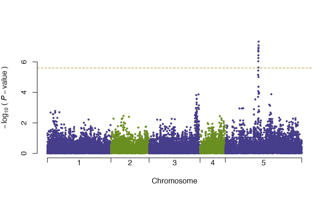
# ----- genomic control ----- #
vgwa2 <- vGWAS.gc(vgwa)

plot(vgwa2)
#> nominal significance threshold with Bonferroni correction for 20000 tests are calculated.

summary(vgwa2)
#> [1] Top 10 markers, sorted by p-value:
#>    marker chr    map             Pval
#> 1  V16630   5 393135 0.00000004639765
#> 2  V16627   5 392704 0.00000008241863
#> 3  V16621   5 391781 0.00000011695436
#> 4  V16614   5 390839 0.00000013025363
#> 5  V16601   5 388736 0.00000017402720
#> 6  V16609   5 390084 0.00000020778158
#> 7  V16612   5 390492 0.00000020778158
#> 8  V16613   5 390663 0.00000036976535
#> 9  V16608   5 389975 0.00000055296825
#> 10 V16598   5 388349 0.00000091305986
# }